image segmentation
scroll ↓ to Resources
Contents
- Note
- Metrics
- [[#Metrics#Technical|Technical]]
- [[#Metrics#Business|Business]]
- U-Net architecture
- Loss function
- [[#Loss function#Integral Image algorithm|Integral Image algorithm]]
- Practical Considerations
- Resources
Note
- Strictly speaking, image segmentation provides per-pixel classification of an image, but it doesn't count objects (like object detection). Therefore, there is an advanced task of instance segmentation uniting the above and which answers both questions: how many objects? and where each of them is located?. instance segmentation architectures though are more complex and data labeling task is more cumbersome.
- Each image in the dataset for image segmentation must have a segmentation map - mapping each pixel to one of the classes or to background. That is contrary to object detection datasets where labeling consists only of bounding boxes’ coordinates for each object.
- ==In 2025 this task is anyway best to solve with self-supervised foundation models with fine-tuning==, not by training from scratch.
- Example applications
- detecting the level of corrosion/rust on the photos of… (e.g. telecom towers, )
- detecting cracks in bridges from drone-made photos
Metrics
Technical
- accuracy - global or class-average
- which portion of pixels do we classify correctly
- global accuracy is not suitable by strong class imbalance
- class-average accuracy does not allow to see the effect of false positives (100% minor class accuracy and 99% accuracy on background class can still be a lot of FP)
- mean intersection over union
- doesn’t show which classes (in case of multi-class) are misinterpreted
- confusion matrix, precision and recall
Business
- depend on the application
U-Net architecture
- U-Net: Convolutional Networks for Biomedical Image Segmentation
- A fully convolutional network architecture from 2015, the name comes from the way layers were drawn in the original paper
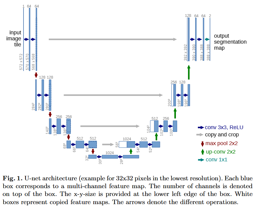
- takes input of 572x572 of black and white images (input tensor depth is 1)
- does not use zero padding to avoid adding noise, when classifying every pixel of an image, which leads to losing 2 pixels after every 3x3 convolution (blue arrows)
- max pooling 2x2 reduces the tensor by 2 (red arrows)
- the deepest tensor in U-Net is 28x28 with 1024 filters (below), after which they apply up-convolution (green arrows) to increase the tensor dimension. 28x28 becomes 56x56
- first, dilation: add zero-rows and zero-columns after each row\column.
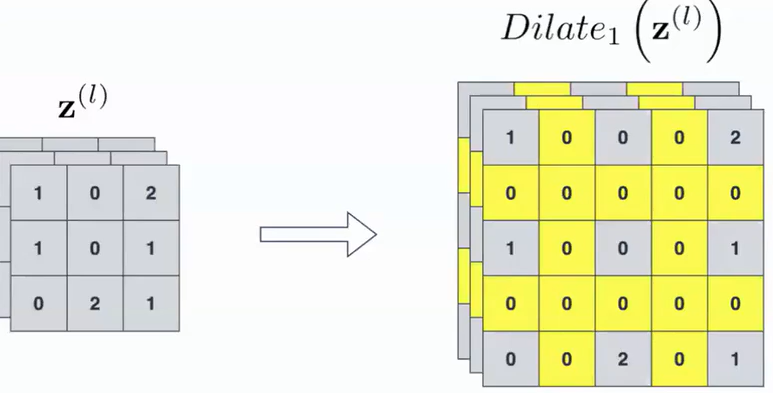
- Second, zero padding and filter 2x2 with step 1, the output is double in size vs the input. This convolution does not learn any features. The up-convolution could be substituted with upscaling\interpolation.
- first, dilation: add zero-rows and zero-columns after each row\column.
- up-convoluted tensor is concatenated (cropping required) with the prior (smaller) tensor (gray arrow). Prior layers (before max pooling) contain more info on geometry and authors combine it with larger receptive field of the latter layers. There are four concatenations.
- Final layer is 388x388xnumber of classes, which is smaller than the original 572x572, that is only central pixels are actually classified.
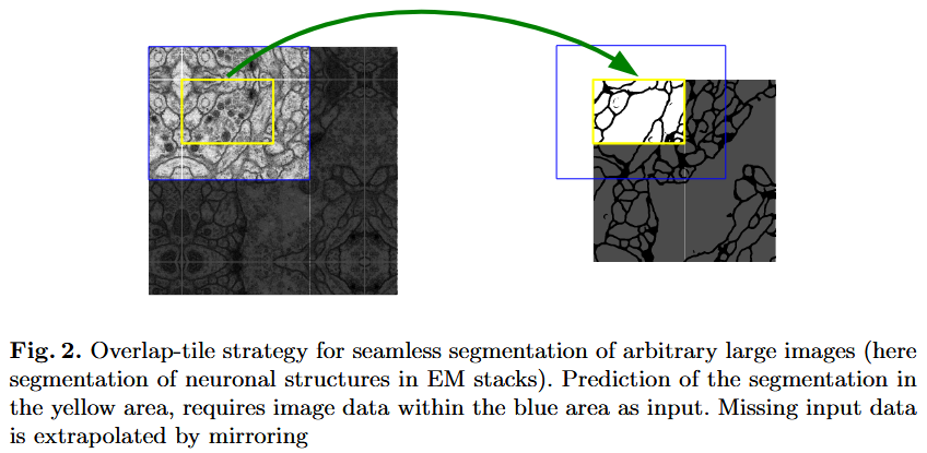
- Normally, raw input images also aren’t exactly 572x572 and rescaling diminishes the purpose of per-pixel segmentation.
- During inference this is solved by smartly cutting raw images into 572x572 with overlap and mirroring on edges (instead of zero-padding).
- All logits go into softmax and total loss is a sum of losses per pixel.
Loss function
- standard cross-entropy for classification, often with class weighting (because it is not possible to control class ratios using batching) averaged over pixels
- class weighting can be
- pre-calculated from the whole dataset (inverse to its occurrence) - does not depict the ratio for any particular image in the training set
- calculated on-the-fly for each randomly sampled 572x572 image (randomly cropped from bigger raw images) - slow and impractical to pre-calculate, because of large number of random crops
- based on Integral Image algorithm
Integral Image algorithm
- how to efficiently calculate how many pixels of a given image belong to each class?
- integral image algorithm does this in 6 arithmetic operations
Practical Considerations
- batching for training set
- in many applications most of the input images will contain only the background class, so all 572x572 pixels belong to one class. It is smarter to sample more interesting parts of the raw image, but it needs to be done on-the-fly. The same calculation, output of the Integral Image algorithm can give an idea if you want to use this cropped image for training.
- receptive field vs Memory Footprint vs Segmentation Resolution
- U-Net with few layers has narrow receptive field. Ability to see larger objects can be done either by down scaling the image (not recommended) or by increasing the number of layers.
- also possible is a custom solution with two network instances with differently-sized inputs. One is learning objects’ features, another only the borders between them. Both outputs are combined and pushed through the final network for actual classification. This system can be trained end-to-end.
- U-Net with few layers has narrow receptive field. Ability to see larger objects can be done either by down scaling the image (not recommended) or by increasing the number of layers.
- technical vs business Metrics
Resources
Links to this File
table file.inlinks, filter(file.outlinks, (x) => !contains(string(x), ".jpg") AND !contains(string(x), ".pdf") AND !contains(string(x), ".png")) as "Outlinks" from [[]] and !outgoing([[]]) AND -"Changelog"