LLM inference
scroll ↓ to Resources
- Note
- Inference engine
- [[#Inference engine#LLM request flow|LLM request flow]]
- [[#Inference engine#Libraries and tools for inference|Libraries and tools for inference]]
- Inference metrics and LLM monitoring
- Inference math
- [[#Inference math#Memory-bound and Compute-bound Programs|Memory-bound and Compute-bound Programs]]
- [[#Memory-bound and Compute-bound Programs#Memory-bound regime|Memory-bound regime]]
- [[#Inference math#Batching|Batching]]
- [[#Inference math#Memory consumption|Memory consumption]]
- [[#Inference math#FLOPs needed to generate one token|FLOPs needed to generate one token]]
- [[#Inference math#LLM throughput|LLM throughput]]
- [[#LLM throughput#The optimal batch size|The optimal batch size]]
- [[#Inference math#Memory-bound and Compute-bound Programs|Memory-bound and Compute-bound Programs]]
- Inference Optimization
- Resources
Note
- Inference process contains three steps
- Downloading the model weights from a cloud storage (Hugging Face) to the drive, where you plan to run your LLM
- Loading downloaded weights into RAM or GPU memory.
- Generating new tokens which are concatenated into the output sequence.
- During the generation step, there are two stages, prompt processing and autoregressive decoding.
- Prompt processing results in the generation of the first token in the output sequence and is generally compute-bound, because of large matrix operations on many tokens in parallel.
- Next, during the autoregressive decoding, tokens are generated one by one. This process cannot be parallelized, so each token is computed sequentially, hence, it is memory-bound The decoding continues until either an End Of Sequence (EOS) token is generated or the maximum sequence length is reached.
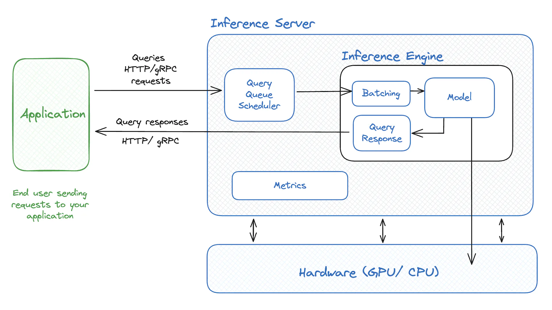
- Inference engine manages the interaction between a user and a hosted LLM.
Inference engine
LLM request flow
Request flow
- The client application formulates a request containing parameters like the input context and generation options.
- The request is sent to the Inference Engine’s endpoint using a protocol like HTTP or gRPC.
- Scheduling and batching: The scheduler queues incoming requests and determines when they will be processed. Requests may be grouped into batches to optimize computational resources. In some cases, a request might be partially processed and then deferred due to resource constraints or scheduling policies.
- Model inference: The model performs a forward pass on the current batch of requests to generate a next token.
- Output processing: The generated tokens are processed and converted into human-readable text.
- The system checks if the generation should stop — either because an End-of-Sequence (EOS) token is generated or the maximum number of new tokens limit is reached. The response is then prepared, containing the generated text and any relevant metadata (e.g., reasons for finishing, token probabilities).
- While the Inference Engine is running, it provides ways to monitor its performance, such as logs or metrics in Prometheus format.
Libraries and tools for inference
- There are numerous tools for LLM inference, perhaps vLLM is one of the best choices for deployment: GitHub - vllm-project/vllm: A high-throughput and memory-efficient inference and serving engine for LLMs
- supports all popular models, including multimodal
- supports quantization out of the box
- built-in monitoring with Prometheus
- API compatible with OpenAI standards
- Deploying vLLM: a Step-by-Step Guide
- But there are other options:
- One can also look at benchmarks: Benchmarking LLM Inference Backends
- Also see the awesome list of all LLM-tools awesome-ml/llm-tools.md at master · underlines/awesome-ml · GitHub
Inference metrics and LLM monitoring
- The most important LLM metrics are
- throughput: the number of requests or tokens an LLM can process per second. Increasing throughput allows the system to handle more tokens and requests in the same amount of time, improving overall efficiency. The peak throughput is the maximum throughput the model can achieve. It depends on several factors, including the model’s architecture, size, and the underlying hardware.
- ==throughput is synonymous to cost in this context==
- latency: the time elapsed from when a user makes a request until the LLM provides a response. This metric is especially critical in real-time and interactive applications, such as chatbots and real-time systems, where quick response times are crucial.
- monitored via LLM metric such as:
- average time for a single end-to-end LLM request in seconds
- Processing speed of input tokens versus generation speed of output tokens as in 3500 prompt tokens per second vs 350 generated ones
- average time-to-first-token in relation to the time required to generate a single output token
- monitored via LLM metric such as:
- Cost: the amount of money spent to process a request. If not completely the same, this is synonymous to the throughput.
- throughput: the number of requests or tokens an LLM can process per second. Increasing throughput allows the system to handle more tokens and requests in the same amount of time, improving overall efficiency. The peak throughput is the maximum throughput the model can achieve. It depends on several factors, including the model’s architecture, size, and the underlying hardware.
Additional metrics
- Time to first token - how long users wait until seeing something
- number of tokens generated per second
- Resource Utilization. GPU, CPU, RAM, Input\Output.
- User feedback in the format of like\dislike or side-by-side model comparison
- Input prompts and their evolution over time, how much are they alike to reference prompts from the test set
- Logs - RAG requests, System I\O, agents’ actions, etc.
- How often a model declines to provide an answer for any reason like harmfulness, security, etc.?
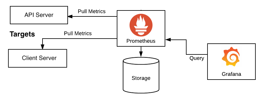
- Prometheus and Grafana are too powerful tools for ML monitoring and visualization
- Prometheus acts as a data collector and a database
- Grafana presents that data in a way that’s easy to understand and interpret
Inference math
Memory-bound and Compute-bound Programs
- Compute-bound program: Its execution time mostly depends on the time spent on calculations (matrix multiplication). To speed it up, one needs a more powerful compute engine.
- Memory-bound program: Its execution time primarily depends on the speed of data movement (matrix transpose). To speed it up, one needs to increase memory bandwidth.
- Certain optimizations, parameters, and hardware used can affect whether the LLM performs in the memory-bound or compute-bound regime. LLM inference is predominantly memory-bound. To improve inference speed, focusing on optimizing memory movement is more effective than enhancing computational performance.
Memory-bound regime
- The time spent on data movement is significantly greater than the time spent on calculations.
- The time for data movement does not depend on batch size.
- Model throughput increases almost linearly, but its latency remains relatively constant.
- However, in the compute-bound area, the throughput remains constant and reaches the peak throughput.
time_of_computations ≪ time_of_data_movements
Batching
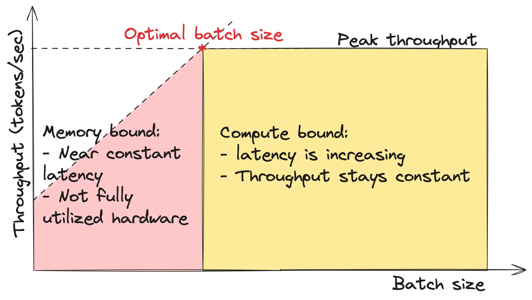
- batch size affects the throughput of the LLM system. When the batch size is small, the LLM operates in a memory-bound regime. As the batch size reaches a certain threshold, the model transitions to a compute-bound regime.
- ==When using batching ALL prompts in each batch must be of the same length==. In LLMs, we use left padding to avoid inserting pad tokens between the prompts and the generation result. This is needed for the correct functioning of LLMs.
- See The optimal batch size below.
Links
-How continuous batching enables 23x throughput in LLM inference while reducing p50 latency
Memory consumption
- LLM weights: for storing all the model parameters. Equals to
num parameters * num bytes per parameter- “small” 8b models in float16 take ~ 15 Gb of GPU memory
- Cache: LLM inference involves multiple passes through the transformer: one for prompt processing and many more for autoregressive decoding. The cache holds intermediate computation results to avoid recalculating them in future iterations. Cache size depends on batch size, context length, and other model parameters.
- Activations: to store intermediate data (neural network activations) during the current iteration of the LLM. Depends on the framework implementation and the floating-point precision used.
- For simplicity, it is sometimes assumed that the context length is small, and hence cache is also negligible, and The activation part remains constant and is also left out of the calculations. Then the memory needed is just
num parameters * num bytes per parameter
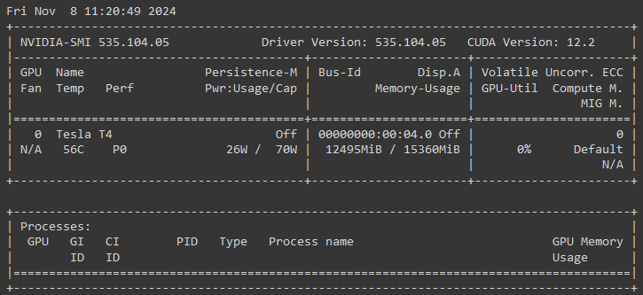
!nvidia-smito check the state of the GPU
FLOPs needed to generate one token
- Roughly speaking, to generate a single token, each token needs to be multiplied by all the parameters and then the results are summed across all parameters.
FLOP = 2 * num_parameters * batch_size * C- C is an additional coeff denoting how many iterations required for one generation. C=1 for text generation, but can be higher for different architectures, image generation like Generative adversarial networks
LLM throughput
time_of_computation = FLOP needed / GPU peak FLOPs = (2 * num_parameters * batch_size) / GPU_peak_FLOPstime_of_data_movement = memory needed / GPU memory bandwidth = (num_parameters * num_bytes_per_parameter) / GPU_memory_bandwidththroughput = batch_size / (time_of_computation + time_of_data_movement)(as in all input tokens divided by the time needed to fully process them)- In memory-bound mode:
throughput(batch_size) = batch_size / time_of_data_movement ~ batch_size / const - In compute-bound mode:
throughput(batch_size) = batch_size / time_of_computation = batch_size * (GPU_peak_FLOPs / (2 * num_parameters * batch_size)) = GPU_peak_FLOPs / (2 * num_parameters)
The optimal batch size
- The optimal batch size is the point on a graph where we can achieve maximum throughput with minimal latency. It is the point where
time_of_computations=time_of_data_movements optimal_batch_size = (GPU_peak_FLOPs * num_bytes_per_parameter) / (2 * GPU_memory_bandwidth)true_optimal_batch_size = min(optimal_batch_size,max_size_that_fits_into_the_GPU_memory)because otherwise it will not fit in the memory, but it doesn’t depend on the model size- For multi-GPU setup, the calculations become more tedious due to data channelling between GPUs.
- In practice, the optimal batch size is much smaller than the theoretical limit due to high memory consumptions of activations and the cache.
Links
- Making Deep Learning go Brrrr From First Principles
- Transformer Inference Arithmetic | kipply’s blog
- Can You Run It? LLM inference calculator
Inference Optimization
Note
Link to original
- use smaller, faster models
- caching ^ef1842
- prefix caching: Paged Attention, vAttention
- Structure your prompt in the way that the most important context is all and changes and additional data appears later
- prompt caching (also partial, in the middle)
- Prompt Cache: Modular Attention Reuse for Low-Latency Inference
- cache identical prompts not to call LLM provider for the same inputs twice
- query caching
- quantization
- By quantizing the model to float16, int8 or int4 is important to check how much the model degrades across different tasks and languages or modalities.
- pruning
- knowledge distillation
- Transferring knowledge from a larger to smaller model
- speculative decoding
- batching
- using different models depending on prompt complexity. Simple question sent to a local model, and complex to ChatGPT
- RouteLLM is a library developing a special router-model to estimate prompt complexity.
- Mixture-of-Experts
- parallelism
- data parallelism - process several documents
- task parallelism - run independent operations at the same time
- make it look faster
- show users intermediate steps
- first provide a rough answer and take more time for refinement and improvement
Resources
Links to this File
table file.inlinks, filter(file.outlinks, (x) => !contains(string(x), ".jpg") AND !contains(string(x), ".pdf") AND !contains(string(x), ".png")) as "Outlinks" from [[]] and !outgoing([[]]) AND -"Changelog"