scaling laws

_{scroll ↓ to Resources}

Note

Methodology from Llama 3 paper

determine compute-optimal models and scaling laws

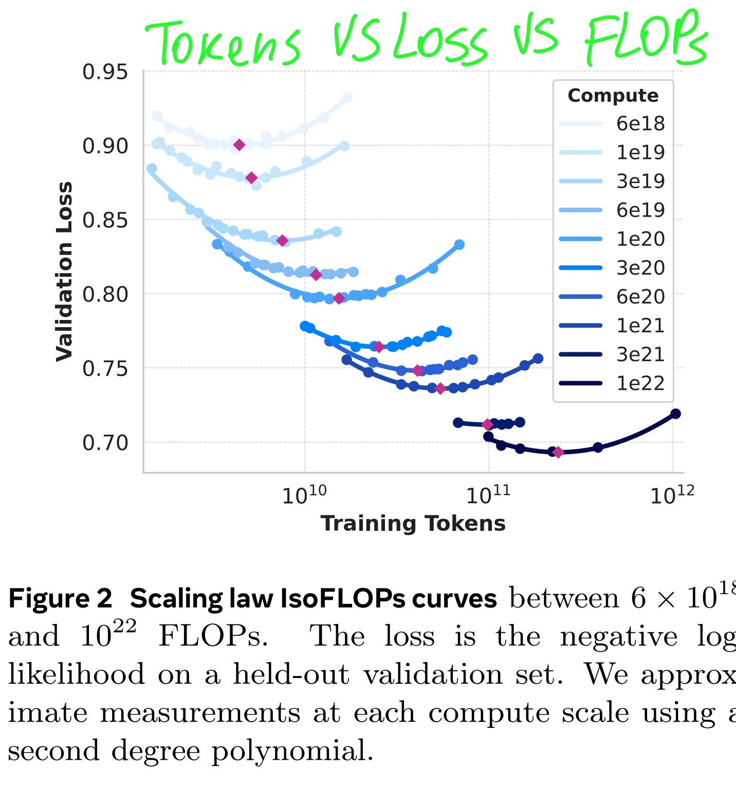
Scaling law experiments. Concretely, we construct our scaling laws by pre-training models using compute budgets between 6 × 10^18 FLOPs and 10^22 FLOPs. At each compute budget, we pre-train models ranging in size between 40M and 16B parameters, using a subset of model sizes at each compute budget

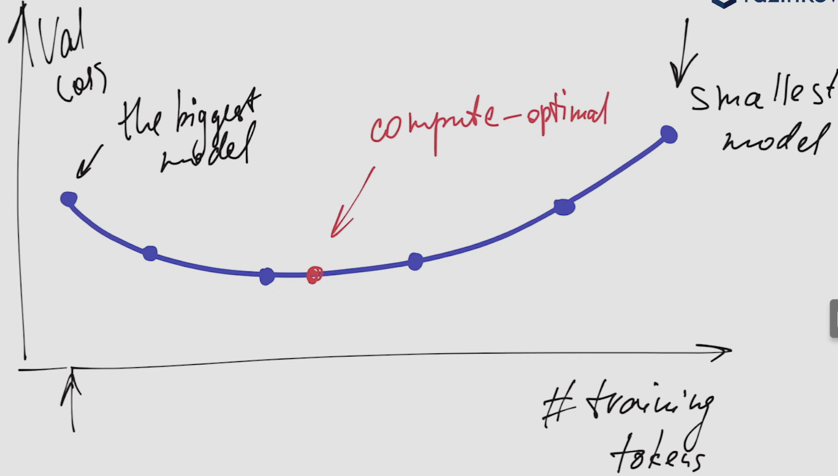
• We create isoFLOPs curves for each compute power and identify the compute-optimal (minimum point) model at the corresponding pre-training compute budget. ==Now we know how many tokens are optimal for each compute budget we used to do these experiments== (this is far less, than the compute budget we are willing to allocate to the final model, but we can’t afford a lot of experiments with that increased budget)

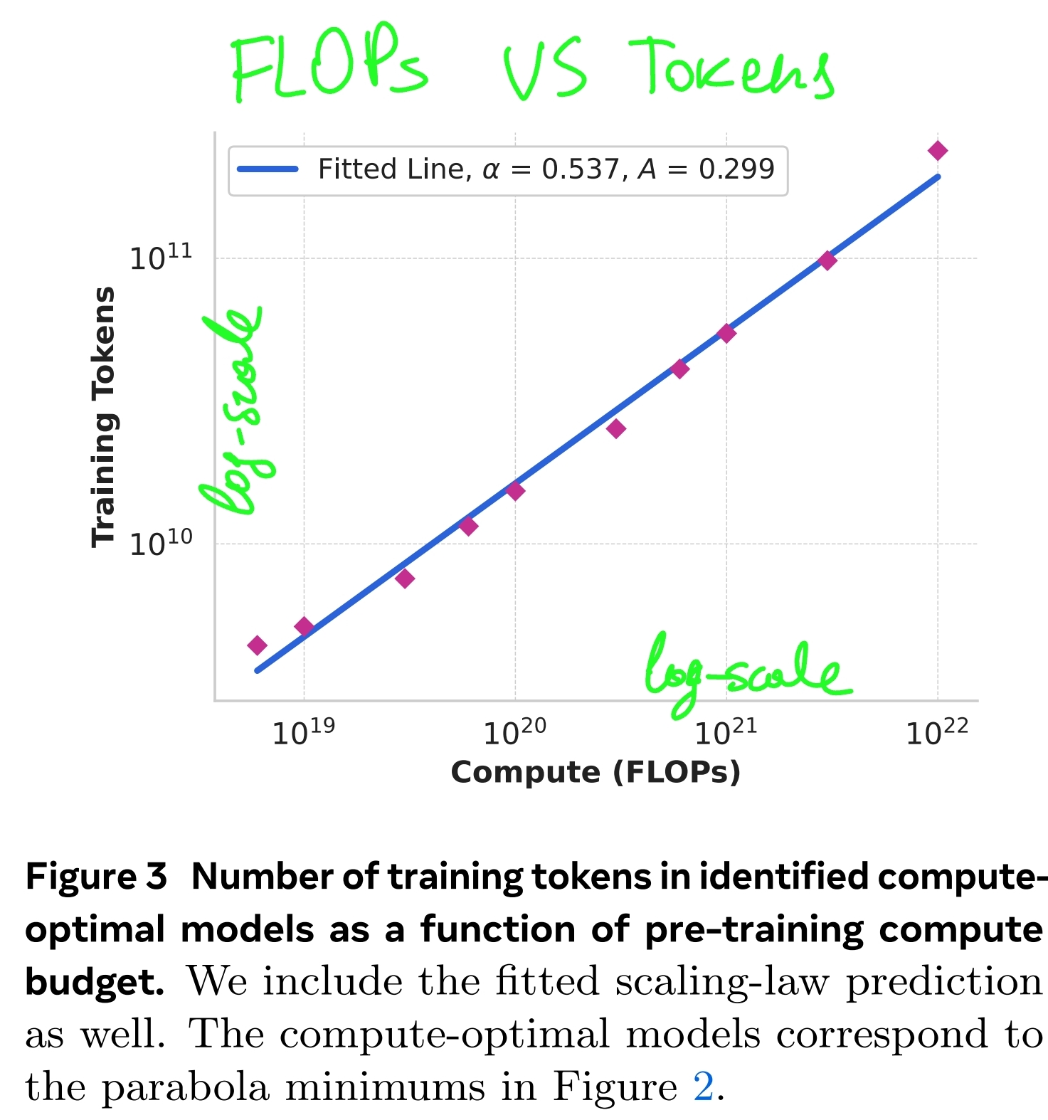
• There is a power-law relation between the number of tokens AND the compute budget which we exploit to determine the optimal number of tokens even for the compute budget we never did any experiments with: $N_{tokens}=A\ast comput{e}^{\alpha }$
  • power-law assumption was established earlier in several papers:
    • Scaling Laws for Neural Language Models
    • Training Compute-Optimal Large Language Models
  • const $A$ and $\alpha$ are fit using compute-optimal data points from experimental isoFLOPs curves

We fit A and α using the data from Figure 2. We find that (α, A) = (0.53, 0.29); the corresponding fit is shown in Figure 3. Extrapolation of the resulting scaling law to 3.8 × 1025 FLOPs suggests training a 402B parameter model on 16.55T tokens.

An important observation is that IsoFLOPs curves become flatter around the minimum as the compute budget increases. This implies that performance of the flagship model is relatively robust to small changes in the trade-off between model size and training tokens. Based on this observation, we ultimately decided to train a flagship model with 405B parameters.

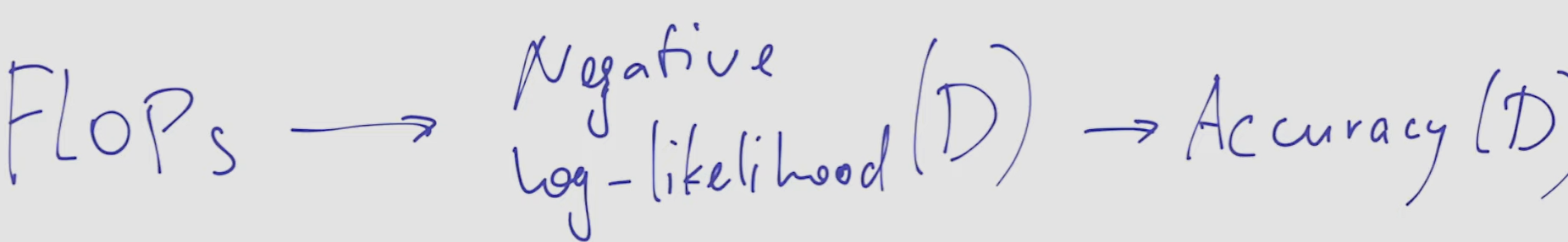
establish a correlation between the compute-optimal model’s negative log-likelihood on downstream tasks and the training FLOPs.

• negative log-likelihood is a next-token-prediction metric: more probable model answers have higher log-likelihood or lower negative log-likelihood

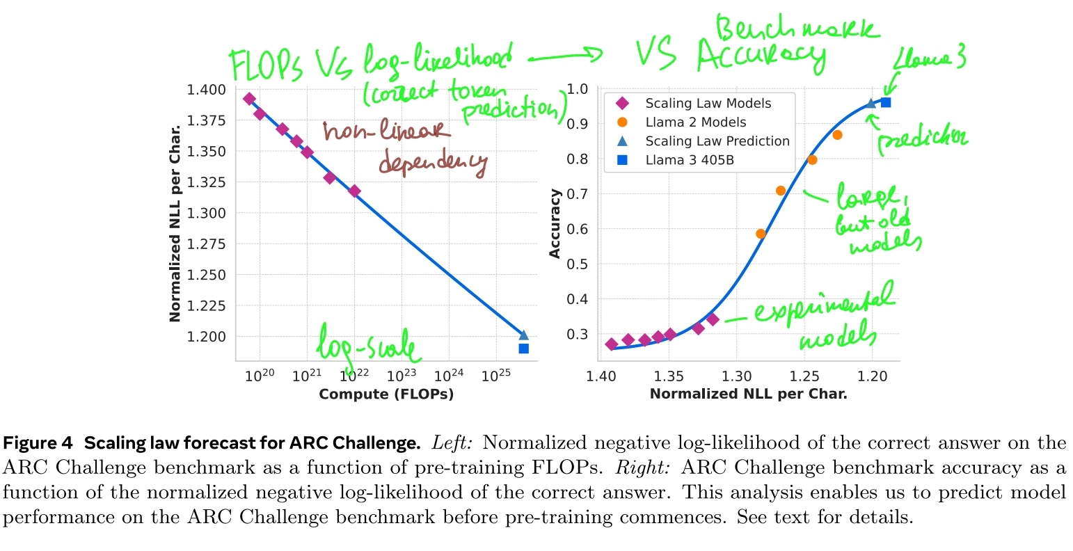
linearly correlate the (normalized) negative log-likelihood of correct answer in the benchmark and the training FLOPs. In this analysis, we use only the scaling law models trained up to 10^22 FLOPs on the data mix described above

• this is dataset-specific dependency

• see left figure in ^0f2352

correlate the log-likelihood on downstream tasks with task accuracy

Next, we establish a sigmoidal relation between the log-likelihood and accuracy using both the scaling law models
and Llama 2 models, which were trained using the Llama 2 data mix and tokenizer.

• so, low-FLOPS models from the above experiments are used together with older top-performance models like Llama 2

final scaling law forecast figure:

Resources

• Scaling_laws_for_LLMs.pdf from Nebius LLM course

---

Links to this File

table file.inlinks, file.outlinks from [[]] and !outgoing([[]])  AND -"Changelog"